Conductivity Tells You One Thing. Impedance Tells You Everything

Part 1 of the Laminar Impedance Series

Most factories already measure the liquids flowing through their pipes — electrically. A conductivity probe, a recipe timer set to a static, worst-case cleaning cycle, and a set of assumptions about what's actually flowing through the line at any given moment. That setup works. Until it doesn't.

A stuck valve. An unexpected soil load. A different product variant. Temperature drift. A partially mixed interface. Or a rinse that looks complete by conductivity but still carries trace residue — a CIP underwash that conductivity alone can't catch. Add SKU proliferation, more variants, more transitions, more edge cases — and that single conductivity value gets stretched further than it was designed to go.

This article is the first in a series exploring the electrical measurement techniques that factories rely on — what they're great at, where they break down, and how "fingerprint-style" sensing transforms visibility for what’s inside the pipes. In future posts we'll go deeper on capacitive sensing, RF and resonant coil methods, inductive (toroidal) conductivity measurements, and more. But first: the fundamentals.

Conductivity Measurement: The Workhorse

A conductivity probe measures how easily current flows through a liquid. Practically, this is driven by ionic content — salts, acids, bases, caustics, cleaners. The probe applies a voltage at a fixed frequency (often around 1 kHz), measures the resulting current, and reports back a single number: conductivity.

Under the hood, this measurement assumes the sample behaves like a pure resistor. Current in, voltage out, done. That assumption holds well for clean ionic solutions, and it's exactly why conductivity is the default sensor in most food and beverage manufacturing CIP loops.

- It's fast, inexpensive, and easy to install.

- It tracks chemical concentration in recirculated solutions reliably.

- It detects gross transitions — water versus caustic, for example — with a clear signal.

- It provides simple pass/fail thresholds for a small number of known states.

If you're running CIP on a straightforward line with a limited product matrix that only requires a simple CIP recipe, conductivity might be all you need for chemical steps. Dosing systems monitor conductivity in the solution tank or return loop and dose chemical to maintain a target setpoint (commonly 30–50 mS/cm for caustic). When conductivity drops below setpoint, more chemical is added.

Where Conductivity Hits a Ceiling

The problem is that liquids in pipes don't always behave like pure resistors. And a single number — no matter how accurately measured — can only tell you so much.

Non-ionic products are invisible. Oils, sugars, and many organic residues don't meaningfully change conductivity. Two very different liquids can look identical to a conductivity probe if their ionic content happens to match.

Interfaces and partial mixing are ambiguous. During a CIP transition — say, going from product to rinse water — the interface between two fluids is a gradient, not a clean cutover. Conductivity can confirm the bulk has changed, but it struggles to confidently call the moment the line is "clean enough" at the boundary. ‍

Temperature dependence is real. Conductivity changes significantly with temperature (roughly 2% per °C for many solutions). Temperature compensation algorithms help, but they add assumptions, and those assumptions can drift.

Air bubbles create false low readings. Air acts as an insulator — it blocks current paths through the liquid, artificially depressing the conductivity reading. Bubbles trapped on the electrode surface are particularly disruptive, as they can significantly alter readings without any change in the liquid itself. ‍

Fouling and cell constant drift. Buildup on electrodes changes the effective geometry, slowly shifting your readings. This is manageable with maintenance, but it's another source of creeping uncertainty.

It collapses the whole picture into one dimension. Even if conductivity is accurate, it can only answer one question: "How ionic is it right now?" It can't tell you what combination of things produces that ionic strength.

This is the core tradeoff. Conductivity is one point on a curve. The natural question is: what would more data points tell you?

Impedance Spectroscopy: Conductivity, but With a Whole Extra Dimension

If conductivity gives you one number, impedance spectroscopy gives you the whole curve.

What Is Impedance Spectroscopy?

Impedance spectroscopy goes by many names depending on the field: Electrochemical Impedance Spectroscopy (EIS), complex impedance analysis, AC resistance measurement, dielectric spectroscopy. But the core idea is always the same — measure the complex impedance at many different frequencies to get a deeper picture of the system than a single-frequency or DC measurement can provide.

Instead of treating the sample as a pure resistor, impedance spectroscopy treats it as a combination of resistors, capacitors, inductors, and even diffusion-like elements — a complex equivalent circuit that changes with frequency.

How Impedance Spectroscopy Works

An electrical system can be tested by applying an input signal — a small sinusoidal voltage — and measuring the output (the resulting current). For a linear, time-invariant system, the relationship between input and output at each frequency can be described by a transfer function. In electrical terms, that transfer function is the impedance Z(ω).

What the System Reveals

When you apply a sinusoidal voltage and measure the current, the system responds with two things:

1. Magnitude — how much the current opposes the flow of current (resistance, in the broadest sense).

2. Phase — whether the current and voltage waveforms are in sync, or whether one leads or lags the other.

That phase behavior is the key. In a purely resistive system, voltage and current are perfectly in phase. In a capacitive system, current leads voltage by up to 90°. In an inductive system, voltage leads current by up to 90°. Real-world systems — including liquids in pipes — are some combination of all three, and the balance shifts depending on the frequency at which you measure.

The impedance of a resistor R is simply R (no frequency dependence). For a capacitor C, it's 1/(ωC) — impedance drops as frequency increases. For an inductor L, it's ωL — impedance increases with frequency.

What Each Frequency Uncovers

By sweeping across a range of frequencies — from millihertz to megahertz — impedance spectroscopy maps out how all these contributions combine. Different physical and electrochemical effects "show up" at different frequencies (different time constants), so the sweep effectively separates:

Bulk electrolyte resistance — the liquid's true conductivity, stripped of everything else.

Double-layer charging — ions queuing up at the electrode surface, acting like a capacitor.

Charge-transfer effects — the friction of electrons crossing from metal into liquid.

Diffusion — how slowly ions can physically move to where they're needed.

Why Frequency Matters: Electrode Polarization

One of the classic problems in electrical liquid measurements is electrode polarization. At low frequencies, ions have enough time to accumulate near the electrode surfaces, creating a large parasitic capacitance that can dominate the measured signal. This isn't an academic footnote — it's a major reason why simple single-frequency conductivity measurements can drift or behave unpredictably outside their designed operating range.

Impedance spectroscopy doesn't magically eliminate electrode polarization. But because the effect changes with frequency, it shows up clearly in the data. You can see it, model it, and compensate for it — often by fitting the spectrum to an equivalent circuit that explicitly accounts for the interfacial capacitance.

How People Visualize Impedance Data

Impedance data is complex — literally, as in complex numbers with real and imaginary parts. There are two standard ways to visualize it:

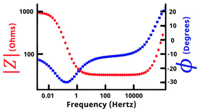
Bode plots show the absolute value of impedance (|Z|) and the phase angle, each plotted against frequency on a log scale. These make it easy to see where the system transitions between resistive behavior (phase near 0°) and capacitive behavior (phase near –90°).

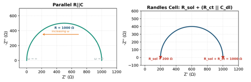
Nyquist plots show the real part of impedance (Z') on the x-axis and the negative imaginary part (–Z'') on the y-axis. Frequency isn't directly visible on the axes — you'd need color coding or labels — but the *shape* of the curve is extremely informative. A classic parallel RC circuit, for example, appears as a semicircle. The diameter tells you the resistance; the frequency at the top of the arc tells you the time constant.

This "shape" becomes the signature of the system. Change the liquid, and the shape changes.

‍

Simulating Impedance Data: Equivalent Circuits

One of the powerful aspects of impedance spectroscopy is that you can simulate (fit) the measured spectrum to an equivalent electrical circuit — a model made of resistors, capacitors, and other elements arranged to represent the physical processes in the system. This lets you extract numerical values for each component, which map to real physical properties.

Take a simple example: a parallel resistor-capacitor circuit. At low frequencies, the capacitor's impedance is very high, so the circuit behaves like the resistor alone — the Nyquist plot starts at the resistor value on the real axis. As frequency increases, the capacitor's impedance drops, eventually shorting the resistor — the Nyquist plot traces a semicircle back toward the origin. Add a series resistance (like bulk solution resistance), and the semicircle shifts to the right.

In real measurement scenarios the curves will be more complex and might not fit a simple textbook model perfectly. But they'll still reveal whether the system is more resistive or more capacitive, and how those behaviors shift with liquid composition.

For applications focused on fingerprinting rather than extracting exact physical parameters, you may not even need the equivalent circuit model at all. You can run calibration samples, build a statistical model, and then apply a calibration curve in the field — treating the impedance spectrum as a signature rather than decomposing it into component values.

What Impedance Spectroscopy Unlocks for Process Liquids

Because impedance changes with frequency, it can separate effects that a single conductivity number collapses together:

- Distinguish liquids with similar DC conductivity. Two solutions might have the same conductivity at 1 kHz but look completely different at 100 kHz or 10 Hz.

- Detect subtle changes in composition, dispersion, or emulsion structure. Changes in particle size, concentration, or dissolved components that don't significantly affect bulk conductivity can shift the impedance spectrum.

- Separate bulk behavior from electrode/interface artifacts. Instead of fighting electrode polarization, you use it as additional information.

The Tradeoff

There's a reason not every pipe already has an impedance spectrometer on it. The electronics are substantially more complex than a conductivity probe. You need a precision frequency generator and phase-sensitive detection across a wide bandwidth — not just a current source and a voltmeter at one frequency. Full spectral sweeps take longer than a single-point measurement, and measurement time scales with the lowest frequency in your sweep (you need at least one full cycle at each frequency to get a reliable reading).

For fast, real-time process control at CIP timescales, this speed-versus-information tradeoff is real.

Resonant Sensing: A Different Path to Spectral Information

There's a middle ground between single-frequency conductivity and full impedance spectroscopy that's worth understanding, because it shows how the same "fingerprint" principle plays out in a different sensor architecture.

Some sensor designs — like those based on resonant LC circuits — use a PCB with a spiral coil (the inductor) and a plate capacitor or interdigitated electrodes (the capacitance). This forms an LC resonant circuit with a characteristic resonance frequency in the MHz range, defined by f₀ = 1/(2π√LC).

How Liquids Shift Spectral Resonance

When this PCB contacts a liquid, the liquid interacts with the electromagnetic fields of both the inductor and capacitor, influencing two things: the resonance frequency shifts (because the liquid changes the effective L and C), and the sharpness (bandwidth) of the resonance dip changes (because the liquid's conductivity introduces losses).

The readout is done using a coupled coil — think of how an RFID tag is read — where a voltage is applied to the readout coil and the reflected power is compared to the applied signal across a frequency range. This produces a resonance curve (closely related to the S11 reflection coefficient used in antenna and RF work) from which two parameters are extracted: center frequency and bandwidth.

In essence, this approach compresses a full frequency spectrum down to two parameters. It's not the full impedance spectrum, but it's substantially more information than a single conductivity value. By plotting resonance frequency versus bandwidth over time, you can perform principal component analysis and distinguish different liquids from one another.

This is a version of the same story that repeats throughout sensing:

- One number gives limited discrimination.

- A curve (or response shape) becomes a fingerprint.

- A fingerprint plus a model becomes classification and control.

The Spectrum of Electrical Sensing Approaches

To put all of this in perspective, here's how the approaches stack up:

Conductivity probe: One measurement at one frequency. Asks: "How ionic is it right now?" Fast, simple, widely deployed. It is necessary but not sufficient to stop timer-based cleaning on its own.

Resonant (LC) sensor: Two parameters (center frequency and bandwidth) extracted from a resonance curve. Richer than a single conductivity value, more compact than a full impedance spectrum. Useful for liquid classification when calibrated.

Impedance spectroscopy: Complex impedance across a full frequency range. Asks: "What physical and electrochemical processes are present?" Powerful for material characterization, but harder to productize for fast inline control.

Each approach lives on a spectrum from simplicity to information density. The question for any factory isn't "which is best" in the abstract — it's "which gives me the information I need to make the right decision at the right speed?"

‍

Where Laminar’s Spectral Sensors Fit

At Laminar, we think about sensing in terms of decisions. The business question during CIP cycles and product changeovers isn't 'What's the conductivity?' It's: 'Can we confidently end this step and start the next one — right now?  

That question demands a sensor signal that is objective (physics-based, not assumptions), continuous and inline (no grab samples or lab turnaround), fast enough to control (sub-second decisions), and auditable (Quality can validate it).

This is why Laminar deploys inline optical spectroscopy — UV/VIS/NIR spectral sensors that read a liquid's spectral fingerprint in the pipe and feed sub-second PLC decisions . Every liquid, soil, rinse, and chemical has a unique spectral signature, and we detect the transition between them in milliseconds.

See how Laminar's spectral sensors and ML models work together on your line: How It Works

Spectral Sensing for Complex Production Lines

Conductivity sensors are good at what they do — and Laminar works well alongside standard instrumentation, including conductivity.  

If you're running a simple line — sparkling water, low SKU count, infrequent changeovers — conductivity may be all you need for your caustic cycles. But if you're manufacturing sauces, syrups, beer, or fragrances, with high changeover frequency, recirculating chemical loops, and organic residues like sugars that conductivity can't see, then conductivity alone is leaving control on the table.  

Laminar's approach adds a higher-information "fingerprint layer" for control, enabling liquid-condition-based CIP rather than timer-based CIP. rather than timer-based CIP.

The electrical sensing methods described in this post share the same philosophical DNA as what Laminar does optically. A spectrum is richer than a single number. A fingerprint drives better decisions than a threshold. The difference is in the modality (optical versus electrical) and the optimization for real-time, industrial-scale deployment.

What's Coming Next in This Series

This post is the broad foundation. In future installments, we'll go deeper into the real-world limits of conductivity, a deep dive into impedance spectroscopy, capacitive and resonant sensing methods, and how electrical and optical fingerprinting come together to enable reliable CIP automation.

Want to keep reading? Don’t miss Jen’s deep dive into spectroscopy.